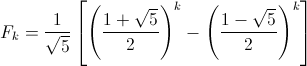
F_k is, of course, the k^th Fibonacci number. Now, before I go on, I want to point out that I stumbled upon these two equations and the proofs for these equations in Gilbert Strang's excellent Linear Algebra and Its Applications. All credit goes to him for coming up with this, and I recommend his book for an even more in depth explanation.

Anyway, back to the equation, which I found interesting for a few reasons:

1. This equation allows you to easily find the kth term using only a pocket calculator. The last equation requires something that can deal with matrices.
2. This also makes it easier to use in programming applications. There's no need to write functions or import libraries to deal with matrices. It's also probably faster than writing some sort of recursive function to compute the kth Fibonacci number.
3. As Strang points out, that equation, amazingly, produces an integer, despite all the fractions and square roots.
4. We can simplify that equation further for a very good approximation (so good that it's not really an approximation).

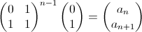
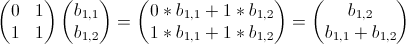
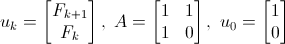
To see how we get that equation from the equation in the last post, let's begin with the way Mr. Strang has it written in his book (it's the same as mine, but flipped upside down).

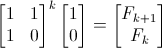
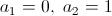
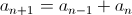
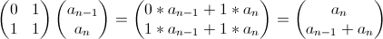
Where F₀=0, F₁=1, F₂=1, etc. Let's now make some substitutions:

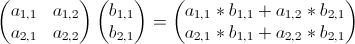
We now have:

This hasn't changed the content of the equation at all. We've just substituted in new symbols to represent the different terms.

The next step is to diagonalize the matrix A. Remember that diagonalizing A produces A = SΛS^-1 where S contains A's eigenvectors and Λ contains A's eigenvalues. Substituting A = SΛS^-1 into the previous equation yields:

Notice how everything but the first and last S and S^-1 cancel, giving the final form: SΛ^kS^-1u₀. This is important, because Λ is a diagonal matrix, making Λ^k very simple:

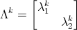
λ₁ and λ₂ are, of course, the eigenvalues of A. Let's now make one last substitution and put all this diagonalization stuff together. First we define c as

Then we substitute it into the equation:

That might need some explaining. The first bit is simply the equation with c substituted in. Following that, the first matrix is S, but written to show that it contains x₁ and x₂, which are the eigenvectors of A placed vertically in the two columns. The middle matrix is Λ^k and the last is simply the matrix c. Finally, the matrices are multiplied out, yielding the final c₁λ^k₁x₁+c₂λ^k₂x₂

The final steps are simply to compute c, and A's eigenvalues and eigenvectors. I'll spare you the tedious algebra and simply tell you that:

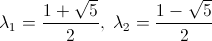
This can be computed the standard way, by solving: det(A-λI)=0.

All the variables are then plugged into the equation for u_k.

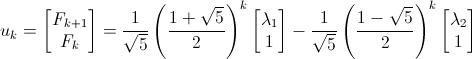
We want F_k, so we multiply, factor, and take the bottom row, giving the equation we want:

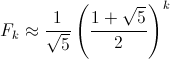
That's the full equation, but now notice that the second term is always less than 1/2. This mean we can simply drop it, yielding:

In fact, since the second term is always less than 1/2 and the full equation always gives us an integer, we can take this a step further: Rounding the approximation to the nearest integer will always give you the exact value for F_k. Cool.

∞ Permalink

That generates the a_n and a_n+1 terms of the Fibonacci sequence.¹ To see why, let's look at a recursive definition of the Fibonacci sequence.

That's easy enough to understand. The first and second terms are both 1, and the next term is the sum of the last term plus the current term. To see how this relates to the matrix above, we must turn this into a matrix equation. The trick here is to have a good understanding of matrix multiplication. If you need a refresher, here's a site with a tutorial. Let's look at an example of a 2x2 matrix multiplied by a 2x1 (even if you have a good understanding of matrix multiplication, hang tight, this is going somewhere).

Now let's make some substitutions and multiply it out:

As you can see, the effect of multiplying the b matrix by the Fibonacci matrix is that it moves the b_1,2 position to the b_1,1 position, and the b_1,2 gets filled with the sum of b_1,1 and b_1,2. Let's now substitute the b's for a_n-1 and a_n:

Does the resultant matrix look familiar? If you look above, you'll see that it's the same as our recursive definition of the Fibonacci sequence! The top row is equal to the current number in the sequence (a_n) and the bottom row is equal to the next number in the sequence (a_n-1 + a_n = a_n+1). Continuing to multiply the resultant matrix by the Fibonacci matrix will cause consecutive entries to be produced. Because matrix multiplication is associative, we can move our multiplication to the exponent, and multiply that result by the first two terms in the sequence (0, 1), leading to our initial matrix:

References

1: Strang, Gilbert. "Linear Algebra and Its Applications."

∞ Permalink